Code
library(keras)
library(tensorflow)
library(grid)
library(gridExtra)
library(magick)
library(viridis)
library(lime)Here, let’s visualise how the Convolution Neural Networks function and learn features of our images !
Here we will visualise the intermediate activations in our model via Feature Maps. This is useful for understanding how successive convnet layers transform their input, and for getting a 1st idea the meaning of individual convnet filters.
library(keras)
library(tensorflow)
library(grid)
library(gridExtra)
library(magick)
library(viridis)
library(lime)We need to disable eager execution to extract gradients later on. Otherwise, the code below will yield an error message stating gradients cannot be processed under eager execution.
tf$compat$v1$disable_eager_execution()model = load_model_hdf5("cats_and_dogs_small_2.h5")
summary(model)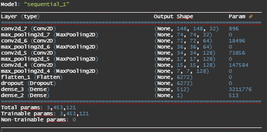
We load two images - a cat and a dog from the test images. First, we convert the images into an array/tensor, reshape it into a specific target size based on our model (here, 150,150,3). Then, we divide the array by 255 to ensure that the range is [0,1].
# picture of a cat and a dog from test images
img_path1 = "C:/Users/KUNAL/Downloads/#R coding/#Books/covered/
#Book - Manning - Deep Learning with R and Keras/cats_and_dogs_small/test/
cats/cat.1591.jpg"

img_path2 = "C:/Users/KUNAL/Downloads/#R coding/#Books/covered/
#Book - Manning - Deep Learning with R and Keras/cats_and_dogs_small/test/
dogs/dog.1535.jpg"

# pre-process the image into a 4d tensor
img1 = image_load(img_path1, target_size = c(150,150))
img_tensor1 = image_to_array(img1)
img_tensor1 = array_reshape(img_tensor1, c(1,150,150,3))

img2 = image_load(img_path2, target_size = c(150,150))
img_tensor2 = image_to_array(img2)
img_tensor2 = array_reshape(img_tensor2, c(1,150,150,3))

# note : The model was trained on inputs that were pre-processed
range(img_tensor1) # range : 2 255
range(img_tensor2) # range : 0 255
img_tensor1 = img_tensor1/255
img_tensor2 = img_tensor2/255
dim(img_tensor1);dim(img_tensor2) # its shape is (1,150,150,3)

# display the input images
par(mfrow=c(2,1))
plot(as.raster(img_tensor1[1,,,]))
plot(as.raster(img_tensor2[1,,,]))
par(mfrow=c(1,1))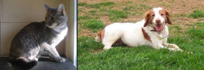
We create a Keras Model which takes as input, images and outputs the activations of all convolution and pooling layers. Here, we have one has 1 input and 8 outputs : one output per layer activation.
#(1) extracts the outputs of the top 8 layers
layer_outputs = lapply(model$layers[1:8], function(layer) layer$output)
#(2) creates a model that will return these outputs, given the model input
activation_model = keras_model(inputs = model$input, outputs = layer_outputs)
#(3) running the model in predict mode
activations1 = activation_model %>% predict(img_tensor1)
first_layer_activation_1 = activations1[[1]] # activation of the 1st conv_layer
activations2 = activation_model %>% predict(img_tensor2)
first_layer_activation_2 = activations2[[1]]
dim(first_layer_activation_1) #it's a 148*148 feature map with 32 channels
# user-defined function to plot a channel
plot_channel <- function(channel) {
rotate <- function(x) t(apply(x, 2, rev))
image(rotate(channel), axes = FALSE, asp = 1,col = terrain.colors(12)) #asp = aspect ratio y/x
}
#(4) Let's visualise the 2nd & 8 channel of the activation of the 1st layer
plot_channel(first_layer_activation_1[1,,,2])
plot_channel(first_layer_activation_2[1,,,2])
#
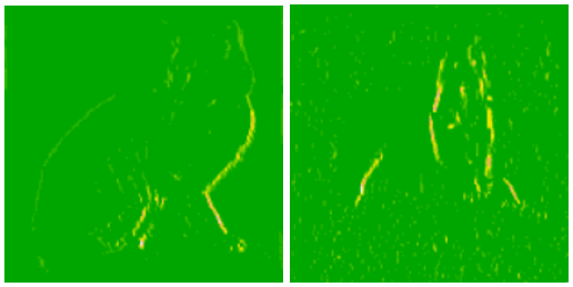
plot_channel(first_layer_activation_1[1,,,8])
plot_channel(first_layer_activation_2[1,,,8])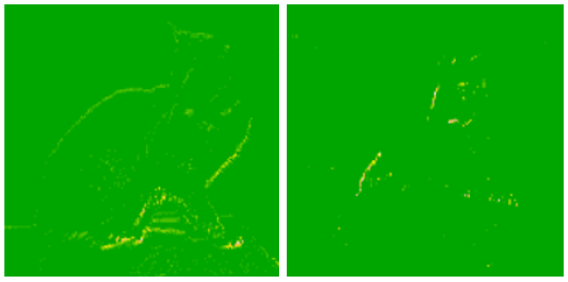
#(5) Visualizing every channel in every intermediate activation
image_size <- 58
images_per_row <- 16

# for loop for Cats
for (i in 1:8) {
  layer_activation <- activations1[[i]]
  layer_name <- model$layers[[i]]$name

  n_features <- dim(layer_activation)[[4]]
  n_cols <- n_features %/% images_per_row

  png(paste0("cat_activations_", i, "_", layer_name, ".png"),
      width = image_size * images_per_row,
      height = image_size * n_cols)
  op <- par(mfrow = c(n_cols, images_per_row), mai = rep_len(0.02, 4))

  for (col in 0:(n_cols-1)) {
    for (row in 0:(images_per_row-1)) {
      channel_image <- layer_activation[1,,,(col*images_per_row) + row + 1]
      plot_channel(channel_image)
    }
    }
  par(op)
  dev.off()
}

# for loop for dogs
for (i in 1:8) {
  layer_activation <- activations2[[i]]
  layer_name <- model$layers[[i]]$name

  n_features <- dim(layer_activation)[[4]]
  n_cols <- n_features %/% images_per_row

  png(paste0("dog_activations_", i, "_", layer_name, ".png"),
      width = image_size * images_per_row,
      height = image_size * n_cols)
  op <- par(mfrow = c(n_cols, images_per_row), mai = rep_len(0.02, 4))

  for (col in 0:(n_cols-1)) {
    for (row in 0:(images_per_row-1)) {
    channel_image <- layer_activation[1,,,(col*images_per_row) + row + 1]
    plot_channel(channel_image)
    }
    }
  par(op)
  dev.off()
}
Here, are all the Feature Maps for our model.
Cat 1591 😼 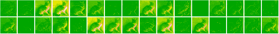 Dog 1535 🐶
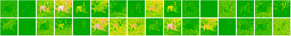
Cat 1591 😼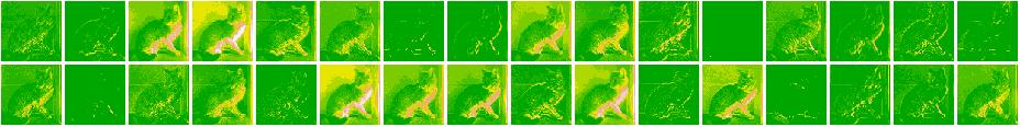 Dog 1535 🐶
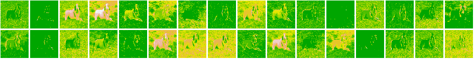
Cat 1591 😼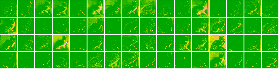
Dog 1535 🐶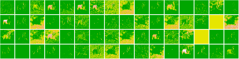
Cat 1591 😼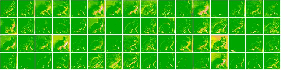
Dog 1535 🐶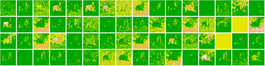
Cat 1591 😼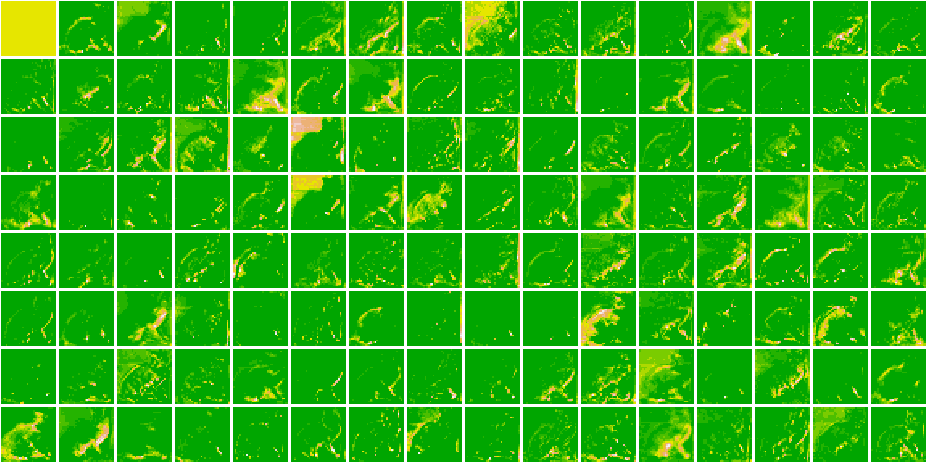
Dog 1535 🐶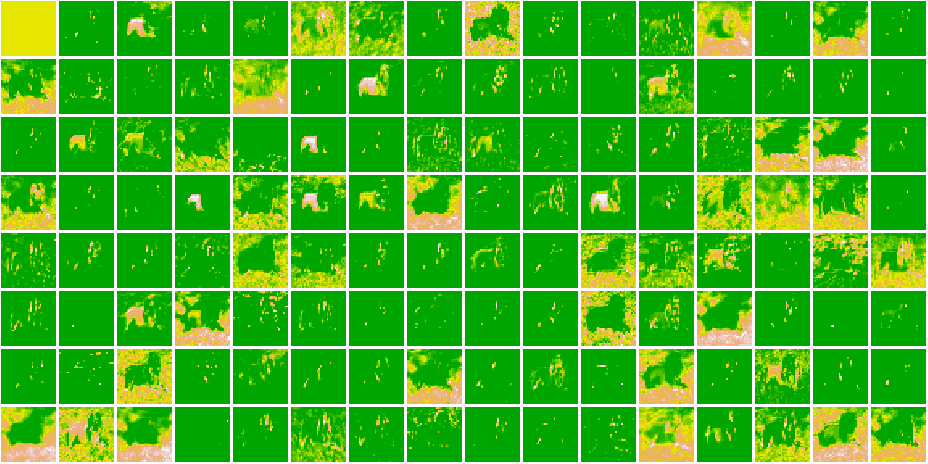
Cat 1591 😼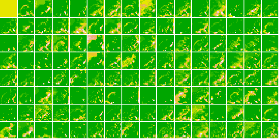
Dog 1535 🐶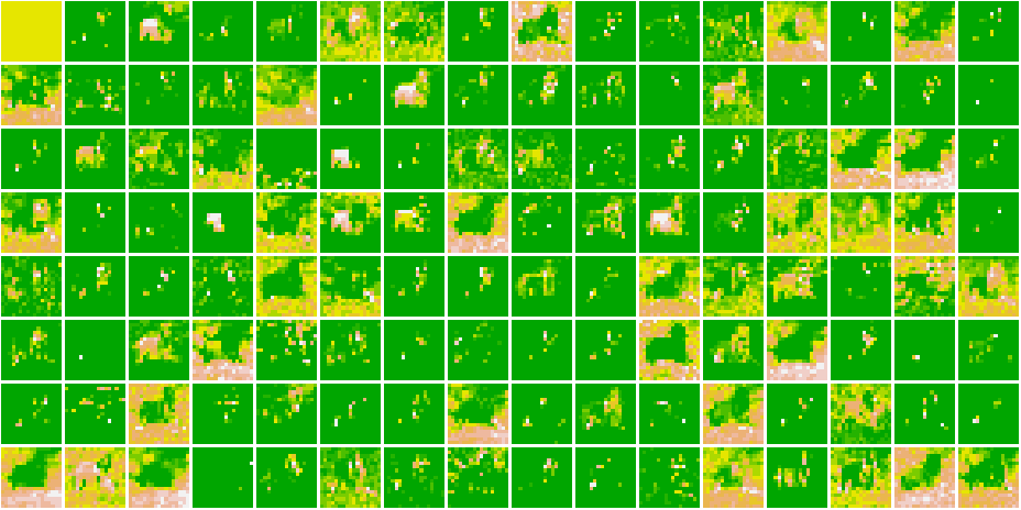
Cat 1591 😼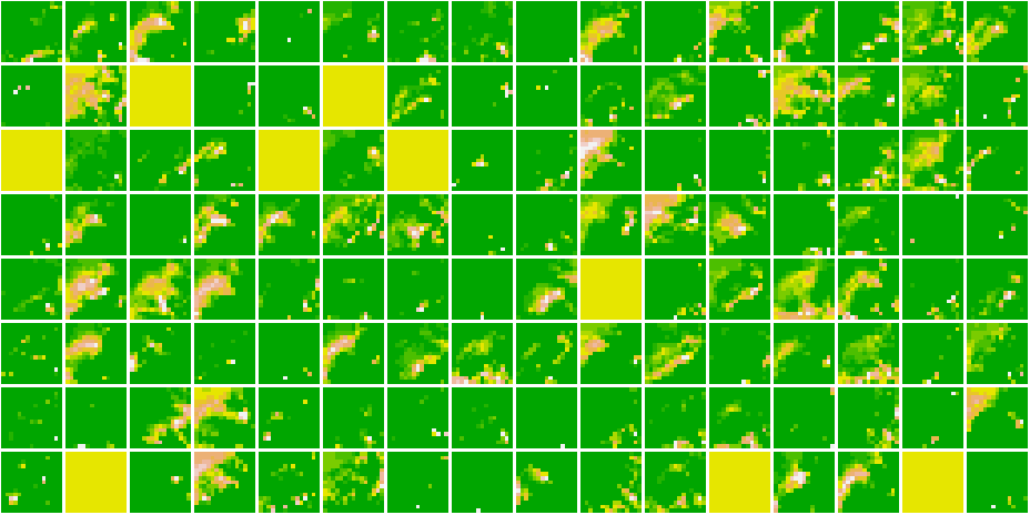
Dog 1535 🐶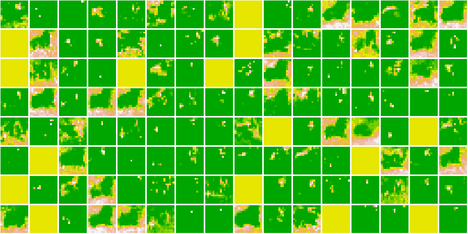
Cat 1591 😼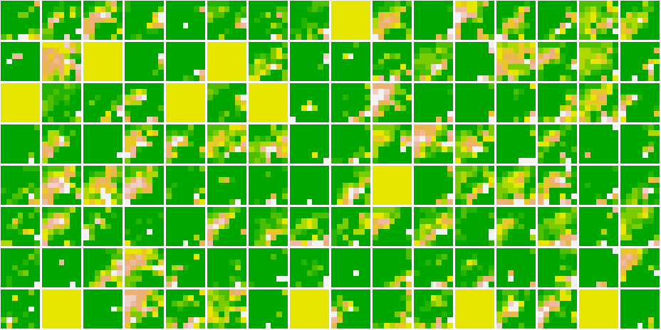
Dog 1535 🐶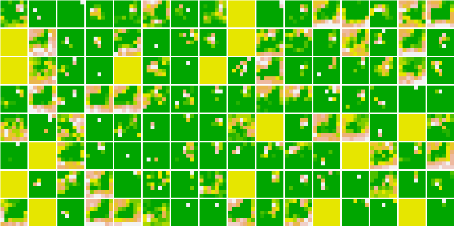
As we go deeper in the network, the features become more and more abstract !
To understand precisely what visual pattern or concept each filter in a convnet is receptive to, we need to plot the convnet filters. This can be done with ‘gradient ascent in input space’ :- applying gradient descent to the value of the input image of a convnet so as to maximise. The response of a specific filter, starting from a blank input image. The resulting input image will be one that the chosen filter is maximally responsive to.
We load Keras Back-end below. Keras Back-end serves as the backend engine of keras. Some operations in Keras require interfacing directly with the functions in the backend engine, and the statement gives K <- backend() us access to those functions.
#(1) load a pre-trained model and a specific layer
model <- application_vgg16(weights = "imagenet",include_top = FALSE)
layer_name <- "block3_conv1"

#(2) load keras Back-end
K <- backend()

#(3) build a loss function that maximises the value of a given filter
# in a given convolution layer
filter_index <- 1
layer_output <- get_layer(model, layer_name)$output
loss <- k_mean(layer_output[,,,filter_index])

#(4) use Stochastic Gradient Descent to adjust the value of the input image
# so as to maximize this activation value. To implement gradient descent,
# we need the gradient of this loss with respect to the model's input.
grads <- k_gradients(loss, model$input)[[1]]
# Note : Gradient-normalization trick :- Add 1e-5 before dividing
# to avoid accidentally dividing by 0
grads <- grads / (K$sqrt(K$mean(K$square(grads))) + 1e-5)

#(5) Fetching output values given input values
iterate <- K$`function`(list(model$input), list(loss, grads))
c(loss_value, grads_value) %<-% iterate(list(array(0, dim = c(1, 150, 150, 3))))
# At this point, we can define an R loop to do Stochastic Gradient Ascent
input_img_data <- array(runif(150 * 150 * 3),
                        dim = c(1, 150, 150, 3)) * 20 + 128
#Starts from a gray image with some noise
step <- 1
for (i in 1:40) {
  # Runs gradient ascent for 40 steps
  # Computes the loss value and gradient value
  c(loss_value, grads_value) %<-% iterate(list(input_img_data))
  # Adjusts the input image in the direction that maximizes the loss
  input_img_data <- input_img_data + (grads_value * step)
}

#(6) De-Processing Function
# The resulting image tensor is of shape (1, 150, 150, 3), with values that may
# not be integers within [0, 255]. So we need to post-process this tensor to
# turn it into a displayable image.
deprocess_image <- function(x) {
  dms <- dim(x)
  x <- x - mean(x)
  x <- x / (sd(x) + 1e-5)  # Normalizes the tensor
  x <- x * 0.1
  x <- x + 0.5
  x <- pmax(0, pmin(x, 1)) # Clips to [0, 1]
  array(x, dim = dms)      # Reshape to original image dimensions
}

#(7) Function to Generate Filter Visualizations
generate_pattern <- function(layer_name, filter_index, size = 150) {
  # Builds a loss function that maximizes the activation of the nth filter
  # of the layer under consideration
  layer_output <- model$get_layer(layer_name)$output
  loss <- K$mean(layer_output[,,,filter_index])
  # Computes the gradient of the input picture with regard to this loss
  grads <- K$gradients(loss, model$input)[[1]]
  # Normalization trick: normalizes the gradient
  grads <- grads / (K$sqrt(K$mean(K$square(grads))) + 1e-5)
  # Returns the loss and grads given the input picture
  iterate <- K$`function`(list(model$input), li*st(loss, grads))
  # Starts from a gray image with some noise
  input_img_data <-
    array(runif(size * size * 3), dim = c(1, size, size, 3)) * 20 + 128
  step <- 1
  # Runs gradient ascent for 40 steps
  for (i in 1:40) {
    c(loss_value, grads_value) %<-% iterate(list(input_img_data))
    input_img_data <- input_img_data + (grads_value * step)
  }
  img <- input_img_data[1,,,]
  deprocess_image(img)
}

#(8) Generating filters for other layers
library(grid)
library(gridExtra)
dir.create("Convnet Filters")
names = c("block1_conv1", "block1_conv2","block1_pool",
          "block2_conv1", "block2_conv2","block2_pool",
          "block3_conv1", "block3_conv2","block3_conv3",
          "block3_pool","block4_conv1", "block4_conv2",
          "block4_conv3","block4_pool")

for (layer_name in names) {
  size <- 140
  png(paste0("vgg_filters/", layer_name, ".png"), width = 8 * size,
      height = 8 * size)
  grobs <- list()
  for (i in 0:7) { for (j in 0:7) {
      pattern <- generate_pattern(layer_name, i + (j*8) + 1, size = size)
      grob <- rasterGrob(pattern, width = unit(0.9, "npc"),
                         height = unit(0.9, "npc"))
      grobs[[length(grobs)+1]] <- grob } }
  grid.arrange(grobs = grobs, ncol = 8)
  dev.off()
}
VGG16 Filters
conv1 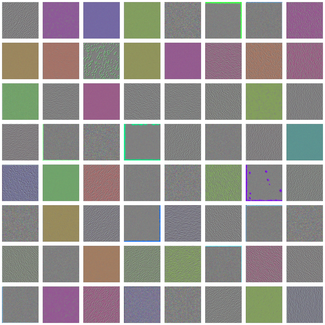
conv2 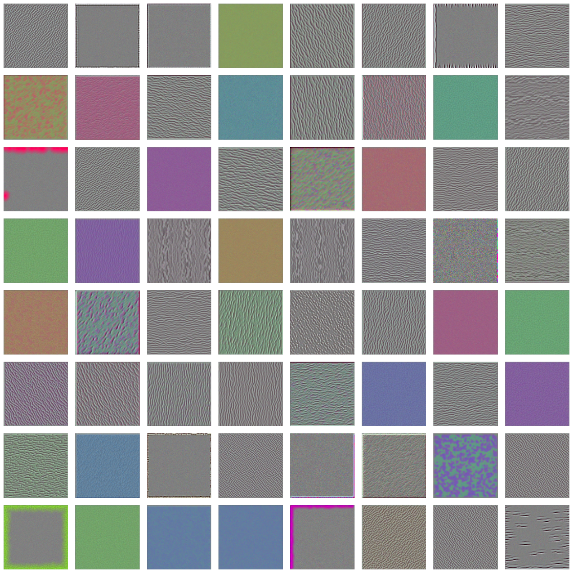
pool 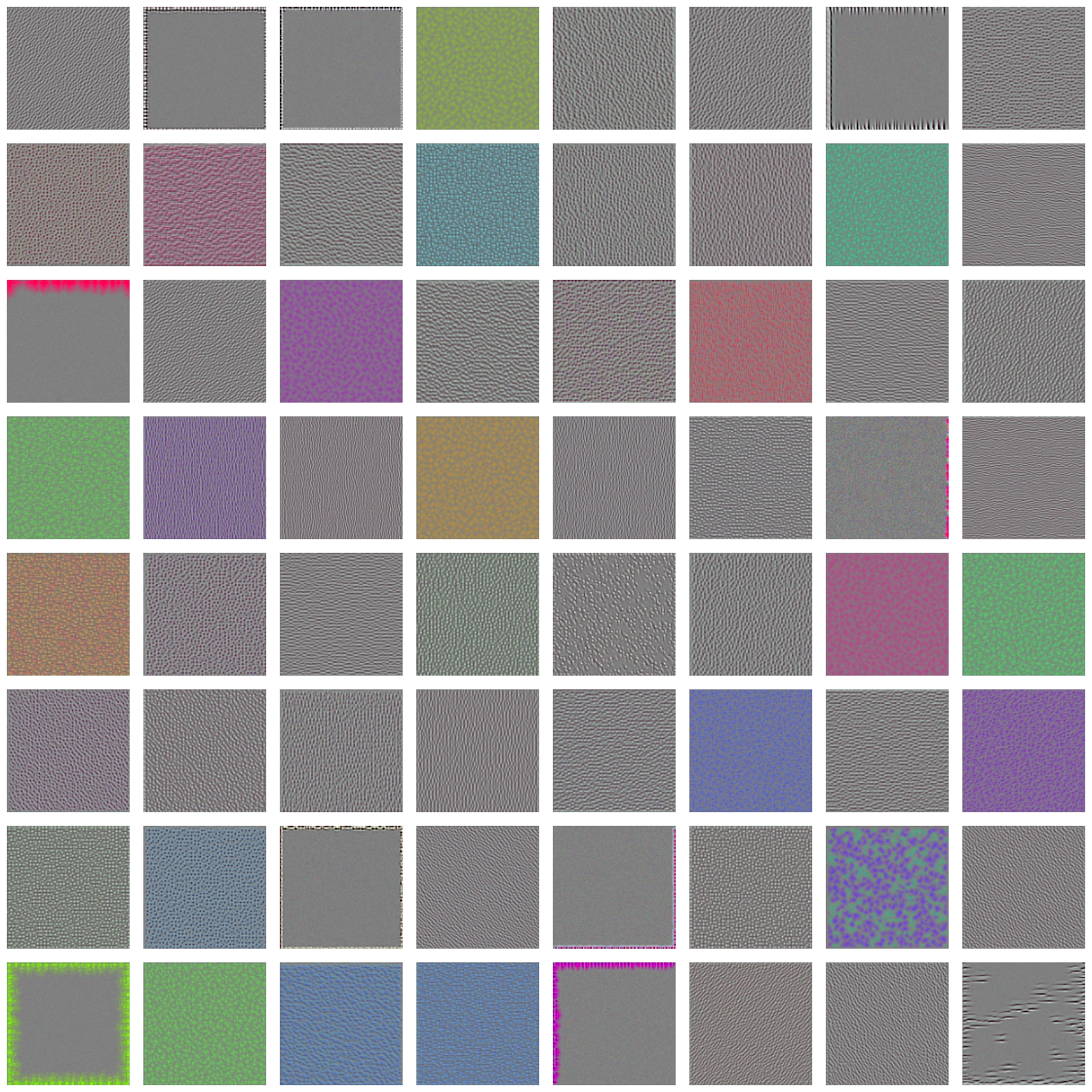
conv1 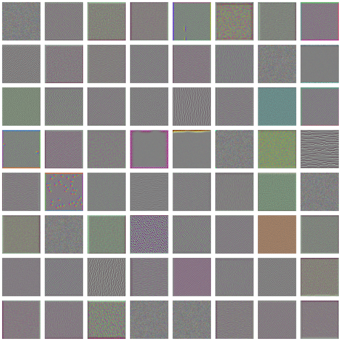
conv2 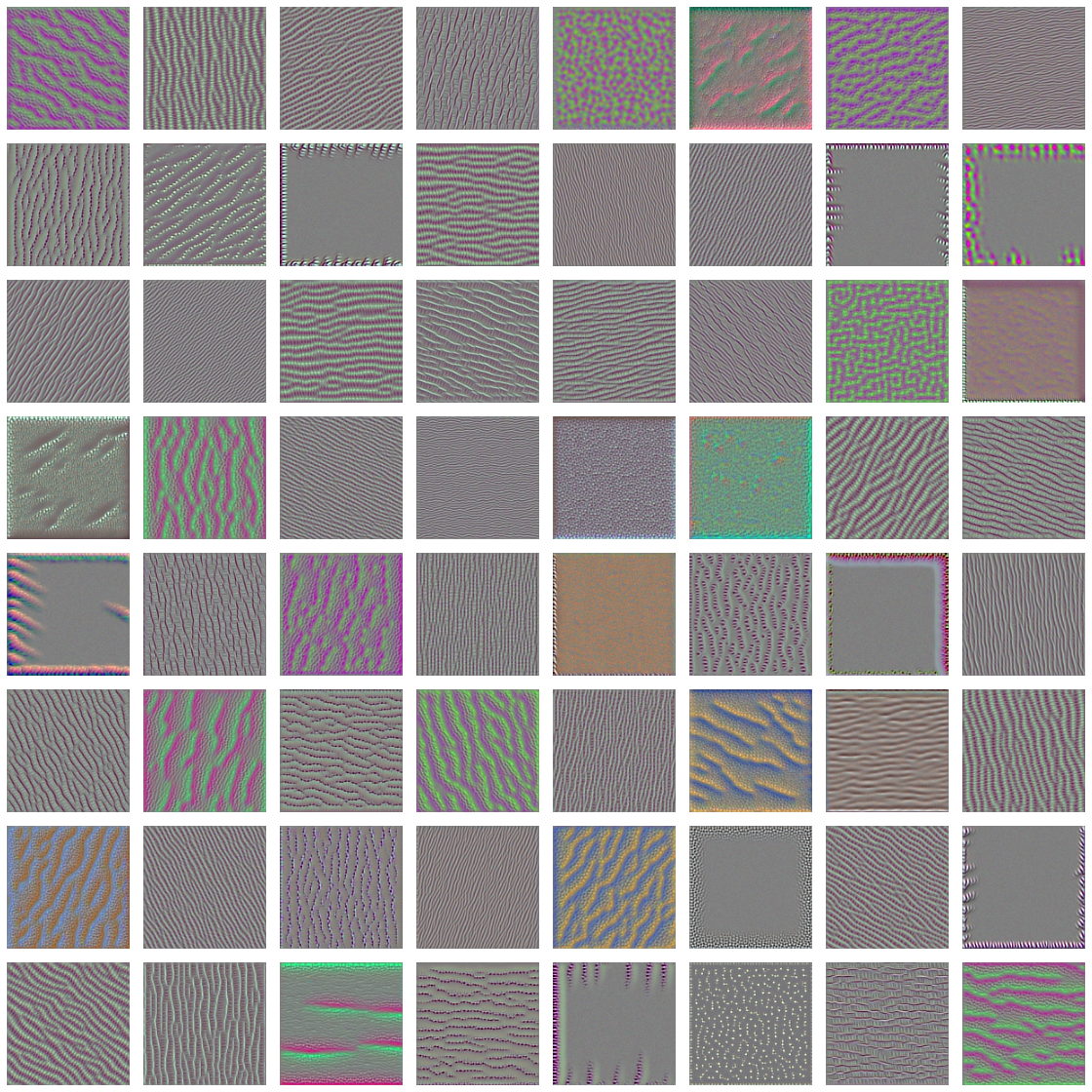
pool 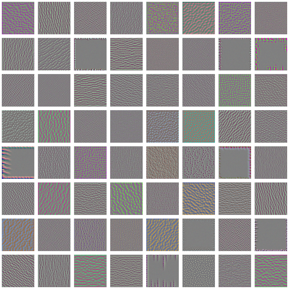
conv1 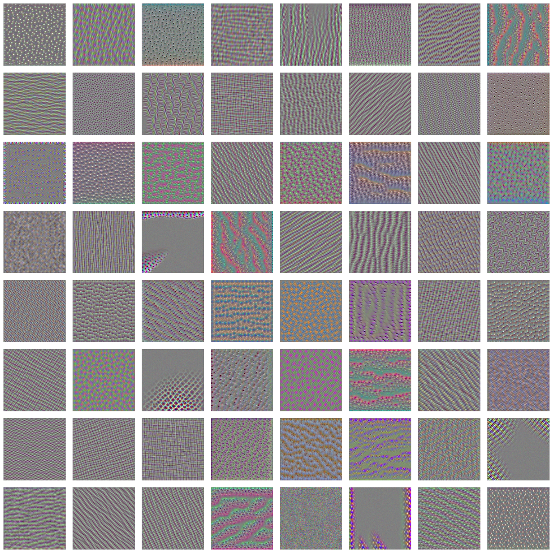
conv2 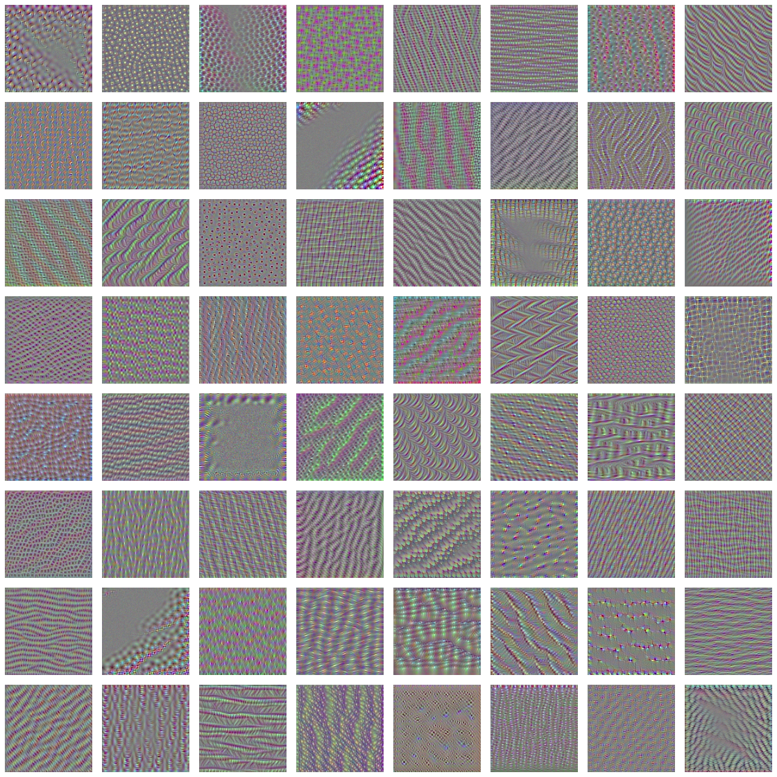
pool 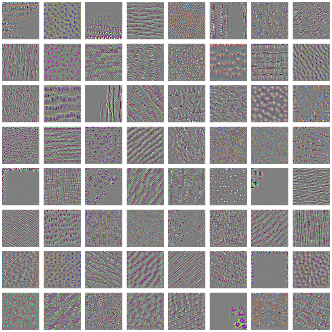
conv1 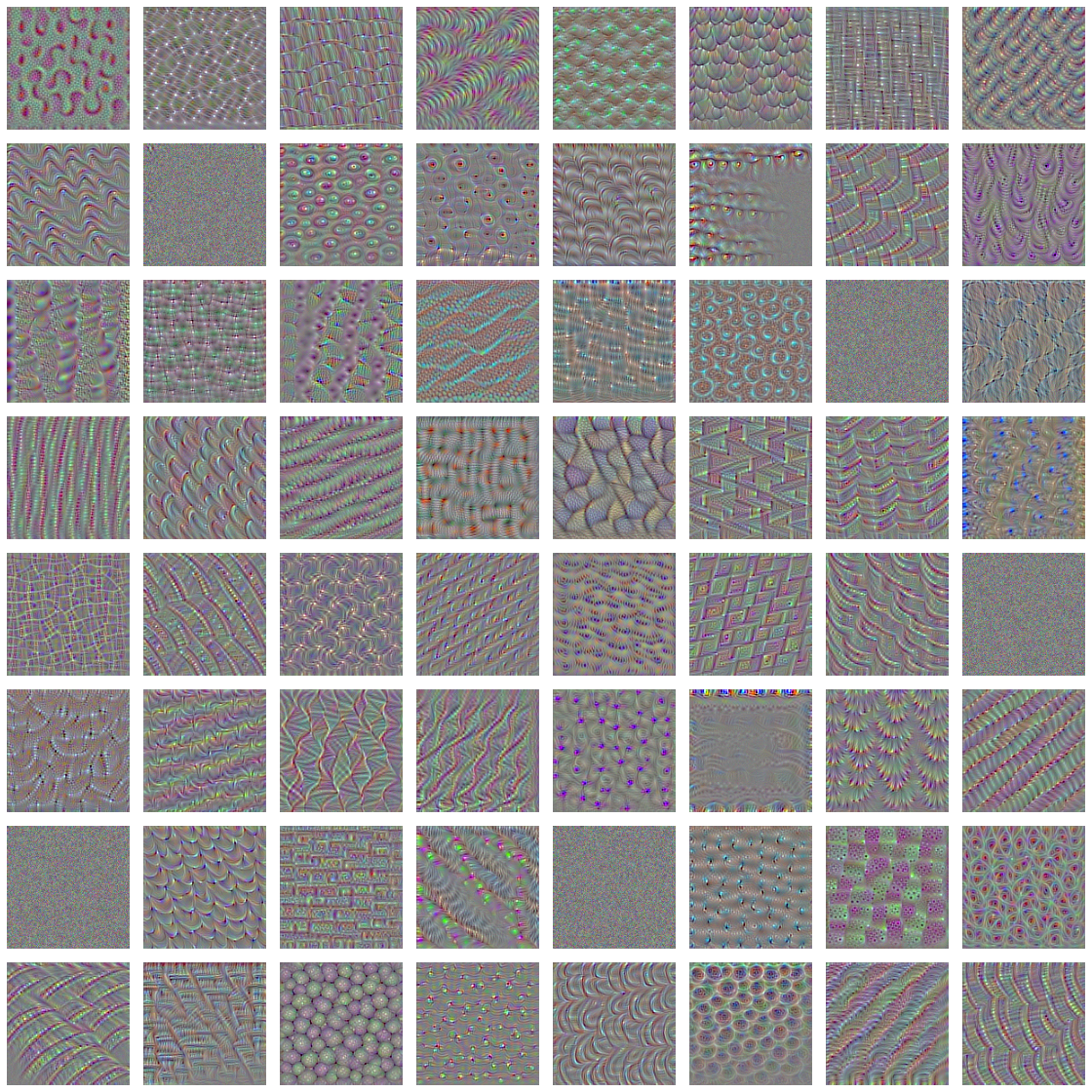
conv2 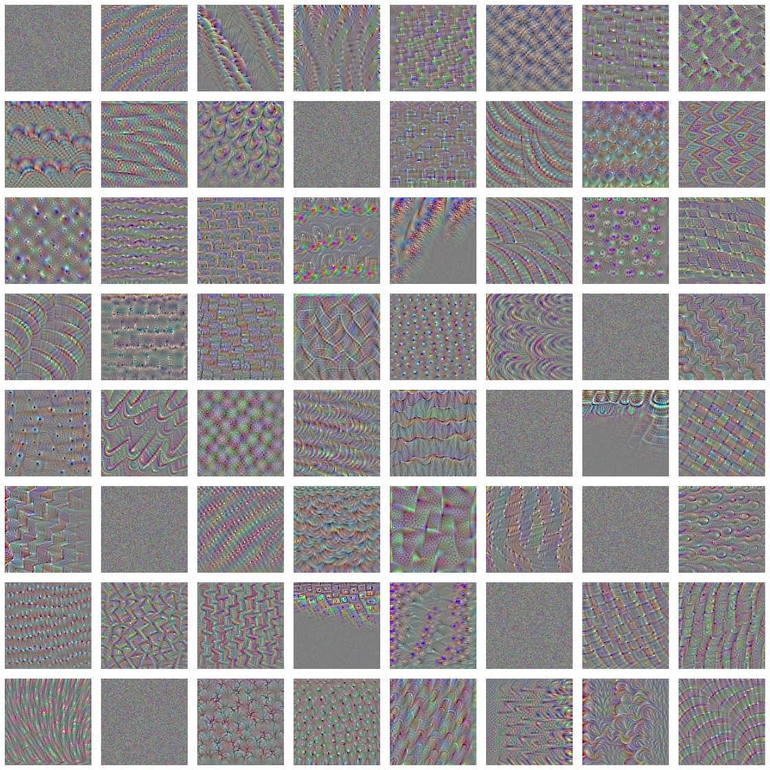
conv3 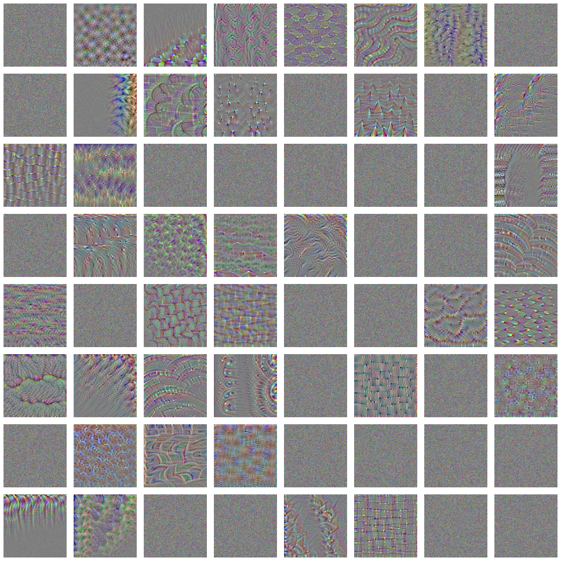
These filter visualizations tell us a lot about how convnet layers see the world:
Each layer in a convnet learns a collection of filters such that their inputs can be expressed as a combination of the filters. This is similar to how the Fourier transform decomposes signals onto a bank of cosine functions.
The filters in these convnet filter banks get increasingly complex and refined as you go higher in the model:
The filters from the 1st layer (block1_conv1) encode simple directional edges and colors (or coloured edges in some cases).
The filters from the 2nd layer (block2_conv1) encode simple textures made from combinations of edges and colors.
The filters in higher layers begin to resemble textures found in natural images: feathers, eyes, leaves, and so on.
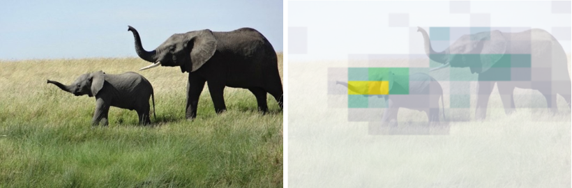
Now let’s visualise the class activations using Heat maps. The idea is to understand which parts of a given image led a convnet to its final classification decision. It is useful for : (a) Debugging in the case of a classification mistake and (b) Locate specific objects in an image.
A class activation map or CAM visualization consists of producing heatmaps of class activation over input images. A class-activation heatmap is a 2D grid of scores associated with a specific output class, computed for every location in any input image, indicating how important each location is with respect to the class under consideration.
Grad-CAM: Visual Explanations from Deep Networks via Gradient-based Localization
It consists of taking the output feature map of a convolution layer, given an input image, and weighing every channel in that feature map by the gradient of the class with respect to the channel. Intuitively, you’re weighting a spatial map of “how intensely the input image activates different channels” by “how important each channel is with regard to the class,” resulting in a spatial map of “how intensely the input image activates the class.”
#(1) Load the VGG16 network with pre-trained weights
model <- application_vgg16(weights = "imagenet")

#(2) Preprocessing an input image for VGG16
img_path3 <- "C:/Users/KUNAL/Downloads/#R coding/#Books/covered/
#Book - Manning - Deep Learning with R and Keras/
creative_commons_elephant.jpg"

img <- image_load(img_path3, target_size = c(224, 224)) %>%
  # Image of size 224 x 224
  image_to_array() %>%
  # Array of shape (224, 224, 3)
  array_reshape(dim = c(1, 224, 224, 3)) %>%
  # Adds a dimension to transform the array into a batch of size (1, 224, 224, 3)
  imagenet_preprocess_input()
  # Pre-processes the batch (this does channel-wise color normalization)

preds <- model %>% predict(img)

imagenet_decode_predictions(preds, top = 3)[[1]]

# African_elephant = 85.62%  # tusker = 13.43%  # Indian_elephant = 0.9332%
# The network has recognized the image as containing an undetermined
# quantity of African elephants.

which.max(preds[1,])
# The entry in the prediction vector that was maximally activated is the
# one corresponding to the "African elephant" class, at index 387

#(3) Set up the Grad-CAM process.
african_elephant_output <- model$output[, 387]
#"African elephant" entry in the prediction vector

last_conv_layer <- model %>% get_layer("block5_conv3")
# Output feature map of the block5_conv3 layer, the last convolutional
# layer in VGG16

grads <- K$gradients(african_elephant_output, last_conv_layer$output)[[1]]
# Gradient of the "African elephant" class with regard to the output

# feature map of block5_conv3
pooled_grads <- K$mean(grads, axis = c(0L, 1L, 2L))
# Vector of shape (512) where each entry is the mean intensity of the gradient
# over a specific feature map channel
iterate <- K$`function`(list(model$input),
# Lets you access the values of the quantities you just defined: pooled_grads
# and the output feature map of block5_conv3, given a sample image
list(pooled_grads, last_conv_layer$output[1,,,]))

c(pooled_grads_value, conv_layer_output_value) %<-% iterate(list(img))
# Values of these two quantities, given the sample image of two elephants
# Multiplies each channel in the feature-map array by "how important this
# channel is" with regard to the elephant class

for (i in 1:512) {
  conv_layer_output_value[,,i] <- conv_layer_output_value[,,i] *
    pooled_grads_value[[i]]
}
heatmap <- apply(conv_layer_output_value, c(1,2), mean)
# The channel-wise mean of the resulting feature map is the heatmap of the
# class activation.

# (4) Heatmap post-processing
# idea : to understand which parts of an image were identified as belonging
# to a given class, and thus allows you to localize objects in images
heatmap <- pmax(heatmap, 0)

# For Visualisation we need to normalize between 0 and 1
heatmap <- heatmap / max(heatmap)

# Function to write a heatmap to a PNG
write_heatmap <- function(heatmap, filename, width = 224, height = 224,
                          bg = "white", col = terrain.colors(12)) {
  png(filename, width = width, height = height, bg = bg)
  op = par(mar = c(0,0,0,0))
  on.exit({par(op); dev.off()}, add = TRUE)
  rotate <- function(x) t(apply(x, 2, rev))
  image(rotate(heatmap), axes = FALSE, asp = 1, col = col)
}
write_heatmap(heatmap, "elephant_heatmap.png")

#(5) Superimposing the heatmap with the original picture
library(magick)
library(viridis)

# Read the original elephant image and it's geometry
image <- image_read(img_path3)
info <- image_info(image)
geometry <- sprintf("%dx%d!", info$width, info$height) # "686x456!"

# Create a blended / transparent version of the heatmap image
pal <- col2rgb(viridis(20), alpha = TRUE)
alpha <- floor(seq(0, 255, length = ncol(pal)))
pal_col <- rgb(t(pal), alpha = alpha, maxColorValue = 255)

write_heatmap(heatmap, "elephant_overlay.png",
              width = 224, height = 224,
              bg = NA, col = pal_col)

# Overlay the heatmap
image_read("elephant_overlay.png") %>%
  image_resize(geometry, filter = "quadratic") %>%
  image_composite(image, operator = "blend", compose_args = "20") %>% plot()
This visualization technique answers two important questions:
In particular, it’s interesting to note that the ears of the elephant calf are strongly activated: this is probably how the network can tell the difference between African and Indian elephants.
Let’s look at how the VGG16 Model performs on our test images.
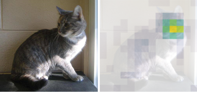
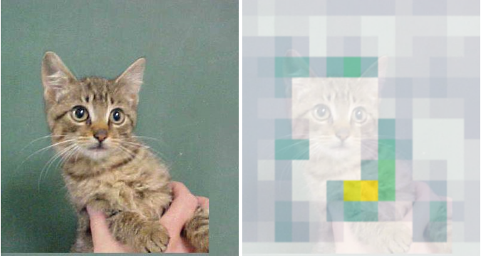
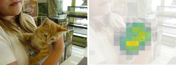
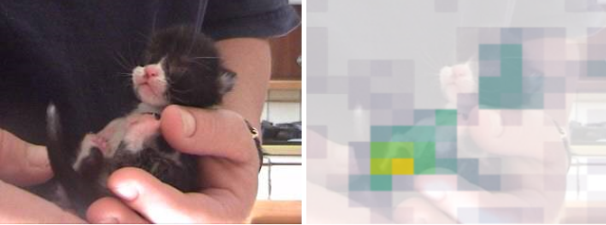
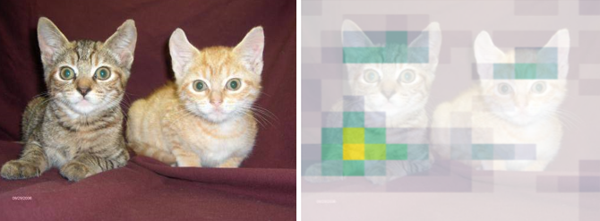
The LIME package offers a simple capability referred to as superpixels. Super-pixels is the process of segmenting an image. We can use this concept to help identify parts of an image that explain our model’s prediction.
plot_superpixels(img_path1)
plot_superpixels(img_path2)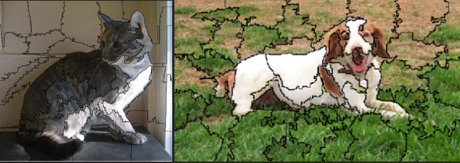
model = load_model_hdf5("cats_and_dogs_small_2.h5")
#(1) function to pre-process an image
image_prep <- function(x) {
arrays <- lapply(x, function(path) {
img <- image_load(path, target_size = c(150, 150))
x <- image_to_array(img)
x <- array_reshape(x, c(1, dim(x)))
x <- x / 255
})
do.call(abind::abind, c(arrays, list(along = 1)))
}
#(2) create LIME explainer
model_labels = c("0"="cat", "1"="dog")
explainer = lime(img_path2, as_classifier(model, model_labels), image_prep)
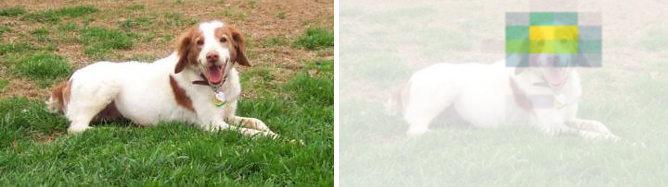
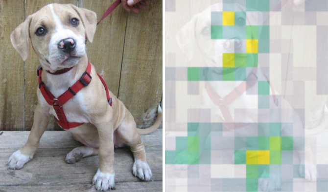
#(3) run the explain() command
# here, we search for 35 superpixels that help explain the model's
# prediction - the current setting uses explanation fit = 0.7 (R-squared)
explanation <- explain(img_path2, explainer,n_labels = 2,n_features = 35,
n_superpixels = 35,weight = 10,background = "white")
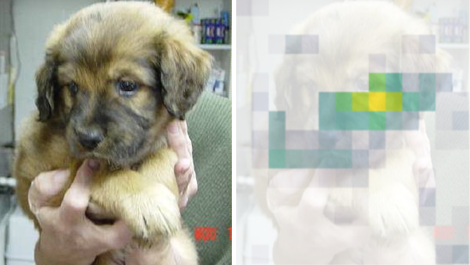
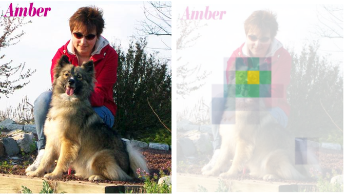
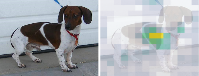
plot_image_explanation(explanation)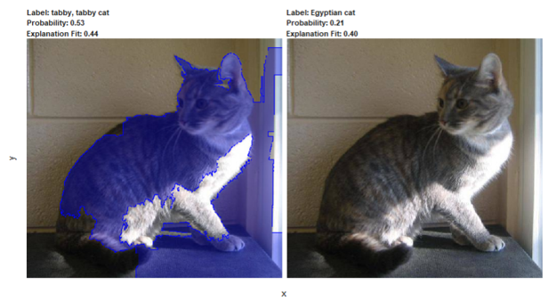
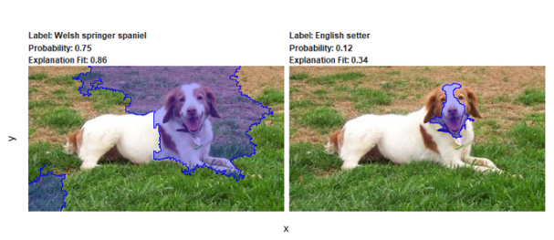
So these are the pixels / area of the image because of which the network is able to confidently classify cats and dogs.
Let’s move on to exploit the power of CNN of real-world issues with Breast Cancer Detection !